

MTO IDF Curves Finder
Dr. R. Soulis, P. Eng.
| Web Page: | Version 3.0 |
| Release Date: | September 2016 |
| Data set: | Environment Canada station data for Ontario, Manitoba, and Quebec up to 2013. The Manitoba and Quebec stations used are within 150 km of Ontario. |
| Version: | IDF v2.3 |
| Date of publication: | January 28, 2015 |
| Number of stations: | 181 |
| Number of station years: | 4562 |
| Data set: |
Precipitation-Frequency Atlas of the United States, NOAA Atlas 14. The NOAA stations used are within 150 km of Ontario. Vol. 2 - Ohio River Basin Vol. 8 - Midwestern States Vol. 10 - Northeastern States |
| Date of publication: | 2006 (Vol. 2); 2013 (Vol. 8); 2015 (Vol. 10) |
| Number of stations: | 171 |
| Number of station years: | 6061 |
| Extreme value PDF: | Gumbel |
| Parameter estimation: | Method of Moments |
| Interpolation Curve: | 2 parameter (A, B) |
| Parameter estimation: | Least squares fit to quantiles |
| Return periods modelled: | 2, 5, 10, 25, 50, 100 year |
| Rainfall durations used: | 5, 10, 15, 30 min; 1, 2, 6, 12, 24 hr |
| Method: | Square Grid |
| Transformations applied: | |
| Independent variables: | None |
| Dependent variables: | log |
| Digital Elevation Model (DEM): | USGS GTOPO-30 |
Ministry of Transportation Ontario
Design and Contracts Standards Office
Drainage and Hydrology Group
Tel.: (905) 704-2293
Intensity-Duration-Frequency (IDF) curves are used in the design
of flood protection infrastructure on small watersheds. They
summarise the annual probability of exceedance,
 , of a
volume of rainfall,
, of a
volume of rainfall,
 (mm), in a single event of duration,
 (hr).
(hr).
 is also known as the probability function,
 , by return
period,
, by return
period,
 (yrs), where:

In this tool, rainfall intensity,
 (mm/hr), is expressed by:

where:

 and
and
 vary with location and return period.
is the value of the IDF curve at the 1 hr storm duration. Since IDF curves
are portrayed as log-log plots, the curves are always straight
lines.
is the slope for each line.
vary with location and return period.
is the value of the IDF curve at the 1 hr storm duration. Since IDF curves
are portrayed as log-log plots, the curves are always straight
lines.
is the slope for each line.
Environment Canada (MSC) publishes
and
parameters at selected
meteorological locations in Ontario and elsewhere in Canada. The
two-parameter form that Environment Canada uses is simpler and
generally more conservative than other forms.
The purpose of this project is to provide a convenient method to interpolate IDF curve parameters between MSC stations for MTO projects.
The method of analysis used is referred to as the Square Grid Technique because it uses UTM grid squares as elementary sub-catchments. The original Digital Elevation Model (DEM) is a set of gridded elevations and drainage fractions coded manually for each 10 km square of the Natural Resources Canada 1:250,000 topographic map series. The current version uses the 30 arc-second GTOPO-30 dataset from USGS.
The premise is that local climate is strongly influenced by local
and regional topography. Thus, topographic parameters are useful
interpolators of surface fields of interest, such as temperature,
runoff and, in this case, IDF curve parameters
and
.
The digital elevation model is used to derive physiographic characteristics that become independent variables in a regression analysis with station statistics. The regression analysis produces a set of generating equations for the parameters used to produce IDF curves. The technique also weighs station data by their length of record, which ensures that data that are more reliable have greater influence on the interpolation. The database consists of statistics from 352 MSC and NOAA stations with an average record length of 30 years.
The result is a gradually varying regional IDF curve. Because the regional curve and station curves both have uncertainty, the regional estimates are different from the station records. However, the 95% confidence intervals overlap and the upper limit is generally higher than the mean station value. Values from both the regional curve and station curves are accessible by this tool.
The minimum recommended design intensities for storms are the values at the 95% upper confidence limit of the appropriate extreme rainfall IDF curve.
The design IDF curve values are the upper 95% confidence limit for the regional prediction, which is generally higher than the station values.
The time trend analysis was done using observations from 1960 to 2014. A linear trend was observed and extrapolated from this period to 2060. Significantly less sources were available for data after 2010, so 2010 is the reference year used in this tool. IDF curve projections are extrapolated from the 2010 base year.
With the exception of the 5, 10, and 15 min storm durations, all t-stats exceed the 95% confidence threshold of 1.96. The lack of significance in these storms is not surprising, as data are more difficult to capture for these events, and the events themselves are less reliable. The t-stats for longer duration events, which range from 2.421 for the 30 min event to 6.979 for the 24 hr event, have a stronger statistical significance.
This project does not address the spatial variability of time
trends for extreme precipitation in Ontario. The analysis combines
the datasets from all stations and determines their collective
historical trend. The projections are extrapolations based on past
trends and assume that the rate of change,  ,
will stay constant. This serves two purposes. For now, the extrapolations provide a better
projection of future precipitation extremes than a stationary
model. In the future, the extrapolation will serve as a baseline
for forecasts that incorporate both climatological factors and
local variability.
,
will stay constant. This serves two purposes. For now, the extrapolations provide a better
projection of future precipitation extremes than a stationary
model. In the future, the extrapolation will serve as a baseline
for forecasts that incorporate both climatological factors and
local variability.
To estimate population parameters of the probability density function, the analysis used the method-of-moments. For the validation, this was compared with an analysis of L-moments. Comparable parameters were generated by both methods.
Rainfall intensities from the 2010 base year are within the safety
margin of previous calculations. Future intensities, however, are
projected to exceed current design standards. The formula for future IDF curve intensities,
 ,
for year
,
for year
 uses the
following equation:
uses the
following equation:

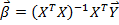
With the introduction of time trends, it is necessary to incorporate a new margin of safety. With the seven independent variables, multiple linear regressions can be performed as shown in the equation below.

in which,
 is the natural log of
parameters generated from the regression analysis,
is the natural log of
parameters generated from the regression analysis,
 is the matrix of the independent physiographic characteristics,
 is the partial regression coefficient vector, and lastly
 is the error vector from the analysis.
With least squares fit,
is found with:
The mean square error is found with:
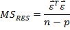
in which,
 is the number of observations in the sample and
 is one plus the number of regression coefficients.
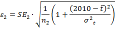
The normalized error,
 , for the mean response is derived with the following formulas:
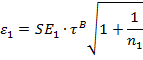

in which,
 is the root-mean-square deviation of the residuals from the regression of
parameters against physiographic characteristics,
is the root-mean-square deviation of the residuals from the regression of
parameters against physiographic characteristics,
 is the rate of change of the rainfall rate per year,
and
is the rate of change of the rainfall rate per year,
and
 is the mean calendar year in the dataset for each storm duration.
The formula for the minimum and maximum intensities to form the confidence interval for the curve uses the following equation:
![R(t)=R(t)*(1[+/-]1.96*e)](graphics/database_status/image033.png)
The approach used in developing the interpolation technique for this tool for Ontario was conceived by the late Dr. S.I. Solomon, a pioneer of distributed hydrologic modelling in Canada, of the University of Waterloo, Department of Civil and Environmental Engineering.
IDF curves from Environment Canada constitute the base data for the interpolation process. These were prepared by Dr. William Hogg and his staff, including Robert Norris and Joan Klaassen, of the Meteorological Service of Canada, who continued the work after Dr. Hogg's retirement.
Project Manager - Dr. Hani Farghaly, P. Eng., Design and Contract Standards, St. Catharines
Project Engineer - Muhammad Naeem, P. Eng., Design and Contract Standards, St. Catharines
Project Science Manager - Dr. Ric Soulis, P. Eng.
Web Interface Design and Construction - Daniel G. Princz, Graduate Student
Database Construction - Dr. Frank Seglenieks, Environment Canada, Burlington
Graduate Student - John (Chon In) Wong
Co-op Students - Jenn Hale, Kaitlyn McIntyre, Setareh Memarian, Daniel Oh, Benjamin Postma, Megh Suthar, Mateusz Tinel, Milos Vojvodic, and Claire Park