Optometrists and ophthalmologists often use a set of features in the eye as an indication of ocular health. These features are usually quantified in some way, and then used for such problems as judging the severity of cataract problems, and measuring irritation caused by contact lenses. There have been many publications detailing the important features of the eye for the latter group [1,2,3,4]; these features have been standardized and a variety of grading scales have been assigned to them. A grading scale is "a tool that enables quantification of the severity of a condition with reference to a set of standardized descriptions or illustrations" [3]. While there is no standard grading scale amongst eye care professionals, there are a few used on a regular basis in many parts of the world [3,4].
Methods of quantifying the set of features relevant to contact lens irritation are very subjective and vary with each practitioner. The most widely adopted method of assigning a grade to a patient is through a comparison of the individual's eye and a set of illustrations or pictures typifying each grade. This method is at best a judgement call on the part of the practitioner and often does not represent the full range of possible grades. This is because the range of assignable grades is limited by the number of pictures that can be conveniently displayed on a reference chart. Given this subjectivity, there exists a lack of consistency in assigning these grades. Grade assignments thus may vary substantially between practitioners.
Our goal is to automate the grading of at least one such feature through processing digital images of the eye. The desired result is user friendly software that will process a digital image of a patient's eye, and provide the practitioner with a grade. Experts in the field of contact lens related eye problems will provide the baseline measurements against which the images will be judged. These tools will enable optometrists and ophthalmologists to standardize their classification schemes for certain contact lens related eye problems.
For the purposes of this paper, it is necessary to define some basic terms relating to the anatomy of the eye. Figure 1 provides a side and frontal view of the eye in which the pupil, iris, fold, sclera and eyelid are identified. The pupil and iris are important to identify in order to locate the centre of the eye; the fold identifies the far edge of the sclera; and the lids border the top and bottom of the sclera. The sclera is the visible white part of the eye. Covering the sclera is the conjunctiva, a thin lining that protects the sclera from disease. Since these are the parts of the eye that a practitioner sees most prominently, we will focus on isolating the sclera and conjunctiva for use in our automated grading system.
The current image-based grading uses either medical illustrations or actual pictures as a baseline. The resolution of these grades is limited by the number of pictures given in the source material. Thus, smaller scales, such as 0 to 4, or 0 to 5 are more popular because they are easier to display. As a result these grades are discrete, and each practitioner must discriminate between fractions of a grade (i.e. what constitutes a 2.5 vs. a 2.25 on a 0 to 4 scale). One scale even suggested counting the number of filled blood vessels to create a more repeatable grading scale [5].
An example of a 0 to 4 clinical grading scale taken from Optician [3] is shown below. This scale demonstrates the crude measures used in clinical practice.
Table 1: Interpretation of Grading Levels
| Grade | Interpretation |
| 0 | Normal - no tissue changes |
| 1 | Trace - clinical action not required |
| 2 | Mild - clinical action may be required |
| 3 | Moderate - clinical action usually required |
| 4 | Severe - clinical action urgently required |
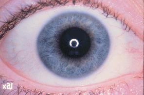
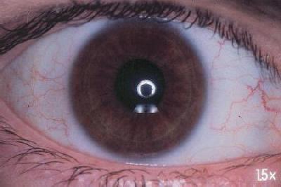
The feature that was examined in the first part of this workshop was that of conjunctival hyperaemia. Conjunctival hyperaemia refers to the presence and abundance of blood vessels in the conjunctiva, the layer of tissue covering the sclera. As an eye becomes increasingly more irritated, the presence and size of blood vessels in the conjunctiva increases correspondingly, resulting in a red appearance. This redness is caused by the eye's immune response to an irritant, either a foreign object or the presence of an irritating solution. For example, while the eye in Figure 2 has very little irritation, the eye shown in Figure 3 shows severe conjunctival hyperaemia.
| Figure 2: A healthy eye | Figure 3: An unhealthy eye | |
 |
 |
We found discussion of automated grading of conjunctival redness in three other papers [6,7,8]; these studies compared the results to a traditional clinical grading as well as assessed repeatability. However, the validity of these programs has never been tested. One paper [7] measured the presence of blood vessels at fixed distanced from the limbus by assuming that the level of redness is proportional to the presence of blood vessels. Unfortunately, this does not provide an accurate picture of the overall redness of an eye, as very fine vessels in the sclera that are normally invisible can also become irritated. Other attempts have tried measures such as the normalized ratio of red to total intensity [6], and total blood vessel area [7,8]. A more recent attempt at automated grading was through the use of morphing to develop a continuous grading scale [11]. The scale was created through the morphing of video clips taken as the redness reaction in an eye diminished.
From these studies, we determined that the important characteristics in determining the severity of conjunctival redness are blood vessel area, overall redness intensity, blood vessel area, vessel diameter, and tortuosity. Since correlating such a large number of features with a clinicians grade of an image would be cumbersome, our efforts have focussed on measuring various dimensions of redness.
Our defined area of concern for the grading of the images is the sclera on both sides of the iris and pupil. This area was chosen because it has been shown that practitioners base their rating of conjunctival hyperaemia (ocular redness) on overall coverage by vessels rather that the appearance of individual vessels [7].
In addition to grading the severity of conjunctival hyperaemia, we will attempt to automatically grade another feature of the eye, as we predict that some of the techniques used to grade conjunctival hyperaemia will be transferable to other clinical scales. Currently, candidates for the second feature include corneal neovascularization and papillary conjunctivitis.
Corneal neovascularization refers to "the formation and extension of vascular capillaries in and into previously unvascularized regions of the cornea" [9]. Since neovascularization also involves measuring the redness in an area of the eye, it is an ideal extension to our previous work. This would allow us to reuse our redness detection software, but require a revision to account for the different area of the eye that we will be examining.. However, since this new area of concern surrounds the iris, it will add the challenge of a variable background colour to our analysis.
Papillary conjunctivitis is the formation and enlargement of bumps or papillae on the eyelid [2,3]. Advanced cases of papillary conjunctivitis have large-diameter papillae, and the eyelid has a bright red/orange hue. Because of the differing diameter sizes of the papillae, the amount of light reflected and way in which it scatters will reflect the severity of the symptom.
Image processing plays an integral role in this project. However, determining the appropriate techniques to use was difficult for this application, since it was necessary to work with colour images. The image processing for this work was completed in MATLAB, using the built-in MATLAB image manipulation functions to read and write images in TIFF format.
The images used for this project were colour images in TIFF format, provided by the School of Optometry at the University of Waterloo. Figures 2 and 3 are examples of these images. These images were taken under controlled circumstances, ensuring that the size, resolution, formatting, centering, and illumination of the eye would be the relatively consistent across images. We could therefore assume certain properties of the images, listed below.
Table 2: Assumed properties of the images
| Property | Value |
| Format | All ocular images will be in TIFF format |
| Location of pupil | All ocular images will be centered on pupil |
| Illumination | All ocular images will be taken under the same illumination |
| Size | All ocular images will be the same size and resolution |
Note that these were not rigid assumptions; we merely used them as guides in developing the software. Whenever possible, the system was designed to operate under conditions that were not as ideal as presented above. For example, the images presented to us were not consistent as to whether the left or right eye was shown. To simplify the initial stage of our work, the images which represented a patients left eye were flipped to ensure that all eyes appeared as if they were the patients right eye. However, the final software will be able to analyse images of either eye.
The general approach we took to solve this problem was to split it up into three independent sections. The first section involved isolating the region to be measured, the second involved taking a redness measure of the region, and the third involved determining an appropriate grade for the image based on the redness measure, given knowledge of how an expert would grade the images.
The details of the methods used in solving these tasks is given in the results section of this report. The basic approach to testing and training can be discussed here: we were provided with 32 images, each of which had two associated grades provided by experts. We used one image as a test image, while the system was trained on the remaining 31 images. This was repeated 32 times, each time using a different image as the control. The grade assigned to the test image in each trial was stored, and when all images had an appropriate grade, the results were compared to those provided by the experts.
There were two development environments under consideration at the start of the project - the xvip toolkit developed at UW for image processing, and MATLAB, a commercially available science/engineering package. The advantages of xvip were that it had some filters already built-in, and it was free. However, it also had many disadvantages: it was not expandable, it was only available in the Apprentice Lab on the UW campus, and the interface to adding new functionality was in C.
MATLAB addressed all of those problems. It already had a large image processing toolkit that shipped with the software, it could run on PCs and UNIX, and the language it used was a C-like language that captured the basic abilities of C without the need for memory allocation, video initialization, and other time-consuming tasks.
We ended up using MATLAB, although the image processing kit was eschewed. It was indeed very powerful, but there was also a steep learning curve that did not justify the extra functionality the toolkit offered.
To properly evaluate of the redness of the eye, it was necessary to isolate a representative region of the sclera. This involved locating the iris, the fold, and the upper and lower eyelids, and removing them from the image. Initially, we attempted edge detection to isolate the iris and eyelids; however, results were poor.
We attempted to detect the iris by performing edge detection in the red plane, reasoning that the iris was never red, and the white of the sclera should therefore contain much more red than the iris. Edge detection using intensity was also performed, on the basis that the sclera would on average have a much higher intensity than the iris. However, both methods of edge detection failed. Although the transition between sclera and iris looks sharp to the human eye, in the image it actually occurred across a gradient of many pixels. This meant that the typical next-nieghbour edge-detection methods were not detecting the change.
While using a larger area (window) over which to measure the difference could have detected this more gradual transition, the resulting edge would have been extremely large. This would have made it difficult to localize the edge with any accuracy.
Detecting the edge of the eyelids was made extremely difficult by the eyelashes, and the redness of the skin. The eyelids broke up the edge with black lines, making it a series of smaller edges, rather than one constant large one. The redness of the eyelid meant that it could potentially be confused with the arteries in the sclera if we did not keep careful track of neighbouring pixels. Even so, the two were still confused in extremely red eyes. These discoveries led us to use a different method for isolating the sclera.
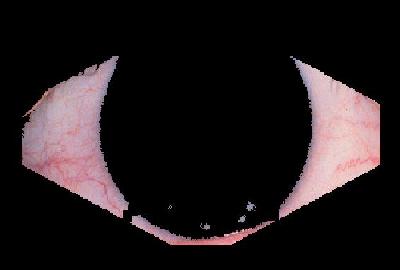
The current method for isolating the shape used for redness evaluation is to use simple colour thresholding to locate the iris, and geometry to remove the eyelids and fold. An example of the desired output is shown below in Figure 6. This shape was chosen because is it the closest approximation to what would be seen by a human observer grading the eye. In theory it will minimize the amount of information lost.
In comparison to the iris and the pupil, the skin and tissue surrounding the sclera has a large red component. This was our most important assumption for the removal of the iris: that the pupil and iris could be distinguished from the sclera and surrounding tissue by their lack of red components.
Based on a straight measure of the percentage of red in a pixel, we removed the pixels that had the bottom 30% of red values. Through experimentation we determined that the top 70% of the red pixels covered the sclera and blood vessels for all of the images. It was possible to achieve near perfect results by removing the bottom 23% of the red pixels for images whose iris was blue. Unfortunately, for brown irises this action removed large portions of the useful information - their red component was too significant to follow our primary assumption.
Many of our images of the eye have a small, white, horseshoe shaped image in the center of the pupil caused by the flash of the camera. To remove this there is a mask that scans the entire image and counts the number of black pixels that lie in the mask. If the number of black pixels is above a set threshold then the entire mask is set to black. Through trial and error, the mask size that produced the best results for all images was a 7x7 mask and the threshold works best at 25 pixels out of 49. A mask size smaller than 7x7 did not remove enough of the illumination in the center, while a larger mask size removed a significant amount of the sclera. The threshold of 25 pixels was chosen since this is approximately half of the total mask size, enough to establish that this area is dark yet also small enough so as to remove large chunks of colour in the center of the image.
Since we found that the straight removal of low-valued red pixels did not work well for brown irises we added the extra mask. An additional run of the 7x7 mask through the full image would cause the loss of information near the black eyelashes. To resolve this problem we ran the 7x7 mask through the center of the image defined by a 120x120 area.
Removing a blue iris presented no problems, as there is very little red in the iris in comparison to the surrounding tissues. However, a brown iris has a much higher concentration of red than does a blue eye. This resulted in a sub-optimal result for the removal of a brown iris if straight redness was used. However, with the 120x120 box removal much of the brown iris was removed. Figure 3 shows the results for one such image.
For the removal of the tissue from the image we assumed some basic things about the image to allow us to remove the surrounding tissue geometrically. The primary assumptions were: the iris is in the center of the image, and all images are approximately the same size.
Based on these assumptions and some experimentation, we were able to determine for one image that there was an outside border of 25 pixels on the image that would not provide useful information. Since we have assumed that all images are of approximately the same size, we extended this assumption to include all images, and a border of 25 pixels wide was created to filter out useless information from all images.
The middle of the image in the x-direction and the middle of the image in the y-direction was found, and these points were then used to make triangles at the corners of the image to remove extraneous tissue. It was experimentally determined that the best results came from connecting points 30 pixels from the center and removing the pixels enclosed in this section, as seen in Figure 6.
For the images that conformed to our assumptions this method of removing extraneous information worked well. However, there was one image for which these assumptions did not hold. For image 16 the iris was far to the left, the method was not flexible enough to recognize this. However, this image can be discarded as a pathological case. Figure 7 shows the results for a more typical image.
Drawing on the hypothesis that the prime factor in an optometrist's categorization is the overall redness of the sclera, we decided upon a pixel-by-pixel operator to measure redness. The input to this system would be the separated image of the sclera from the isolator program, with the output being a vector of floating-point values representing different redness measurements.
For the remainder of this section, we will use P to represent the score a metric gives a pixel, OUT to represent the overall output for an image, and RGB will be the red, green and blue components of a pixel.
There are two ways a TIFF image can be stored, packed and unpacked. In the unpacked format, each pixel is represented by a 3x1 vector of integers with values ranging from 0 to 256. The elements in the vector represent the RGB components of the pixel, respectively. In the packed format, each pixel is represented by an index into a colourmap, where the colourmap is an array of RGB vectors specifying every colour represented in the image.
The images we were working with were all in the unpacked format. While this type of image consumed more space, they were much simpler to process. We will assume that all images input into the system will be in this unpacked format.
There are several measurements that can be made on a pixel to determine its "redness". We wanted a measure that would produce output that was consistent with the optometrists' grading. It was also important that the results were reasonably spread out; the more tightly grouped they were, the more likely that noise would corrupt our grading.
The first and most obvious measurement that we considered was measuring the average value of the R component of the image. However, this was dismissed without implementation, because it fails to differentiate between pure red pixels and those that have high levels of G and B as well.
The next measurement we considered was the percent redness of the image, via the formula
Black pixels were ignored, both because the edge detector coloured non-important pixels black, and to avoid divide-by-zero errors.
In the end we rejected this measurement, because it gave the same moderate redness rating for any pixel that was close to greyscale (R=G=B). This means that even though red pixels would give a P score of around 1, many of the white pixels in the sclera would also score around P=1/3. While it would be simple to correct for this, the measurement still does not separate out our P scores as much as we would like.
The next measurement we considered was the average difference between the R and G values of the pixels (ignoring black pixels), using the formula
The logic behind this measurement is that the part of the image that we will be examining (the sclera) will be a white background with red foreground. Any other colours will be either noise, or deviant cases. Using the formula, white pixels will give P=0, while pure red pixels yield P=256. Purple pixels (R=B=256, G=0) would also yield P=0, but as mentioned before purple pixels are not likely to occur in the sclera. Because of this separation of the outputs, the RG difference was the primary metric we used in grading the images.
We also considered measuring the average red-blue difference, using the formula
In an ideal situation this metric would yield the same results as the RG difference. In practice it would be valuable when there was some corruption in the green plane (such as an overall green tint) which would cause the previous metric to produce skewed results. The RB difference could be used as a backup measure, averaging it with the RG difference. In the graph below, we compare the RG difference with the RB difference for a series of test images. As expected, they are very closely correlated except for image 25, which has a blue tint overall.
The red detection algorithms were run on a series of test images created by manually blacking out the parts of the image which were not sclera. The results are shown below in Table 3. The image numbers for each grading metric and for the optometrists are listed in descending order of redness (the most red image is listed first). TLS and TC are the rankings given by two optometrists, R-perc is the Percent-Red metric, and RG-diff is the Red-Green Difference metric.
We can see that the automatically generated rankings are generally in line with the optometrists', although they do not align perfectly. For example, image 16 was ranked as the most red image by both of the optometrists and the red-percent metric, but the red-green difference metric ranked it second. Note that this table only gives the rankings; the actual scores - and thus the separability - are not represented.
Some deviance from the grades provided by the optometrists is expected because of two problems with the images used. Variation in illumination levels in the images affected the results of some images, while the presence of colour noise, such as the blue tint in image 25 skewed results for others. Automatic detection and correction of these types of problems will be part of the focus of future work.
Table 3: Red-detection rankings vs optometrists' rankings| Rank | TLS | TC | R-perc | RG-diff |
| 1 | 16 | 16 | 16 | 18 |
| 2 | 29 | 29 | 18 | 16 |
| 3 | 15 | 15 | 15 | 15 |
| 4 | 18 | 18 | 29 | 29 |
| 5 | 05 | 05 | 05 | 05 |
| 6 | 12 | 12 | 09 | 04 |
| 7 | 09 | 28 | 04 | 09 |
| 8 | 27 | 03 | 28 | 30 |
| 9 | 28 | 09 | 27 | 10 |
| 10 | 03 | 30 | 12 | 03 |
| 11 | 14 | 27 | 03 | 06 |
| 12 | 30 | 14 | 30 | 12 |
| 13 | 08 | 08 | 08 | 14 |
| 14 | 04 | 04 | 06 | 08 |
| 15 | 02 | 13 | 10 | 28 |
| 16 | 17 | 10 | 14 | 27 |
| 17 | 25 | 02 | 13 | 31 |
| 18 | 32 | 32 | 01 | 01 |
| 19 | 10 | 25 | 31 | 13 |
| 20 | 07 | 07 | 21 | 07 |
| 21 | 31 | 31 | 24 | 32 |
| 22 | 01 | 17 | 32 | 24 |
| 23 | 23 | 01 | 02 | 17 |
| 24 | 06 | 23 | 07 | 21 |
| 25 | 21 | 21 | 23 | 23 |
| 26 | 22 | 11 | 17 | 11 |
| 27 | 24 | 22 | 11 | 02 |
| 28 | 26 | 26 | 22 | 22 |
| 29 | 11 | 06 | 26 | 19 |
| 30 | 20 | 20 | 19 | 26 |
| 31 | 19 | 19 | 20 | 25 |
| 32 | 13 | 24 | 25 | 20 |
When we ran the original red detection program on the images, two types of noise were found to be interfering with our results. The first was the variance in the images' illumination level, and the second was colour wash.
In some of the images the illumination level was slightly higher or lower than the rest of the images. This caused our metrics to give these images P-scores that were skewed from the ones they should have received. To correct for variations in lighting level, we must multiply the image score by some correction factor. As of yet, this feature has not been implemented. Even without it, the correspondence between the program's scores and the optometrists' scores is reasonable. This is because the pictures were all taken under the same general lighting conditions.
There is also the problem of images that have been tinted by some colour. For example, image 25 had blue noise evenly spread through the sclera, seen in Figure 5. This resulted in the RB difference metric being significantly different from the RG metric. To correct for colour noise, we need to re-establish our baseline of "white". One suggested method is to measure the luminance of all the pixels of in the sclera, and average the top few percent to get our new measure of whiteness. Again, this feature has not yet been implemented.
For the images provided, grades were obtained from Trefford Simpson of the Optometry department. To obtain a grade for each image, we used the grades of all the other images in the test set to train the system. For each of these images, the redness was calculated and compared to the professionals' grading. The polyfit function was used to fit a 2nd order polynomial curve to the results of our redness as compared to the practitioners grade.
Then for each test image, the polyval function was used to determine it's location on the curve from our redness calculation. round was then used to determine the nearest grade, an integer result. This resulting integer was our grade, which was then stored. When the system had tested each image and returned a calculated grade, the calculated grade could be compared to the practitioners grade for each image to determine the accuracy.
Ideally, more options would be considered for the curve fitting, for example, linear, exponential or logarithmic curves, as well as 2nd order polynomials.
In this section we will discuss what future work needs to be done on this project, the desired final product, and an approximate time line for completion. The first step is to consider how the current state of the project compares to what we projected we would have completed by now.
In our problem statement at the beginning of this project, we stated our goals for the project for this point in time: we hoped to have developed a basic hypothesis for how practitioners would grade an ocular image, and some basic MATLAB routines to simulate it. This hypothesis included the general region of the eye to examine, and a theory regarding the specifics of redness measured. Finally, we planned to have a prototype that could test our tools, and some results to see if our initial hypotheses were generally correct. As discussed in the results section of our report, we have achieved these goals.
Our goal for the completion of this project is to have user friendly software that produces a grading for redness that is objective and repeatable, and consistent with the grades that would be produced by an practitioner who is an expert at clinical grading. We would also like the software to be able to handle another type of clinical grading, either bumpiness or neovascularization. This would enable us to test the applicability of our work to a wider range of clinical grading problems.
To complete this work, we must perform the following tasks over the next four months:
With these goals in mind, the following simple timeline has been developed for the progression of future work on this project.
Table 4: Revised timeline for the next 4 months| Dec. 15 - Jan. 5: Improve shape isolation and redness measurement routines; develop faster, more efficient code | |
| Extracting grades, general algorithm, test results | Cindy |
| Redness Routines | Vikas |
| Shape isolation with user input | Shannon |
| Jan. 5 - Jan. 31: Test shape isolation, redness separately, try different measures | |
| Optimize software | All |
| Develop GUI, write front end | Cindy |
| Feb. 1 - Mar. 1: Research into other grading applications | |
| Research methods of bumpiness/neovascularization | All |
| Develop prototype grading scheme for alternate features, if feasible | All |
| Mar. 1 - Mar. 31: Test Software and Document Results | |
Our work to date on this project has provided us with valuable insights in the areas of image processing and clinical grading. While the work on this project done thus far has focused on creating a simple system, the software will serve as a base for a more robust system to be developed in the future. In its current state, our software will isolate the sclera from an ocular image and assign it a grade. It works well for certain images, but our work for next term will focus on modifying the software to handle a wider variation of images.
We discovered that edge detection was a false avenue and decided instead to use colour gradients to isolate the sclera in the image. Our results were very good for some pictures, but barely acceptable for others. Future improvements to the isolation of the shape via user input should improve these results. For grading these images, it seems that the red-green and red-blue differences produce the most promising results. However, they still do not correspond completely to the grading provided by expert practitioners, so more research needs to be done. We will also implement luminance and colour noise correction routines.
Maintained by Vikas Nagaraj